
Generative AI
Can a 4B Model Match a 14B Model? We Fine-Tuned 8+ Models to Find Out
Key takeways from fine-tuning 8+ language models on a text classification task, from tiny 0.6B models to 14B behemoths.
December 5, 2025

Bauke Brenninkmeijer
Research Engineer

Key Takeaways
Fine-tuned Qwen3-14B achieved 93.4% accuracy (beating 100B+ base models)
Prompt engineering delivered +34% accuracy, equivalent to 5-10x model scaling
LLM labeling works: $26 for 8,000 labels with dual-model approach
We spent weeks fine-tuning 8+ language models on a text classification task, from tiny 0.6B models to 14B behemoths. The question:
Could a well-tuned small model match, or beat, models 10x its size?
The answer surprised us, and the lessons learned apply far beyond our specific use case. While we do our best, this is not an academic paper, but rather a practical, empirical account of what we tried, what failed, and what you can apply to your own fine-tuning projects.
Glossary
This post assumes familiarity with ML fundamentals (training/validation splits, classification metrics) and basic LLM concepts. Here’s a quick glossary:
Term | Definition |
|---|---|
Parameters (4B, 14B) | The number of learnable weights in a model that roughly correlates with capability and cost |
Fine-tuning | Training an existing model on task-specific data to improve performance on that task |
LoRA | Low-Rank Adaptation, which trains only 1-5% of model weights, dramatically reducing memory and compute requirements |
Prompt engineering | Designing input text/instructions to improve model output without changing model weights |
The Business Need
At Orq.ai, we process thousands of conversational traces daily. Understanding what users are discussing (technology questions, business inquiries, creative requests) can give valuable insights to clients. Manual classification doesn’t scale. We needed automated topic classification that’s fast, accurate, and cost-effective.
The Technical Challenge
Text classification sounds simple until you try it. We started with 7 main categories (Technology, Science, Arts, Economics, Personal Development, History, Other) and initially attempted 56 subtopics. The boundaries are fuzzy: is “AI ethics” Technology, Science, or Personal Development? Is “startup funding” Economics or Technology?
Our Goal
Could we fine-tune a 4B or 14B parameter model to beat larger base models? If so, we’d get faster inference, lower costs, and the ability to self-host. The prize: production-quality classification at a fraction of the cost.
The Baseline: What We Were Trying to Beat
We chose the Qwen3 model family for a specific reason: it offers a wide range of sizes (0.6B to 235B) within the same architecture. This let us isolate the effect of model scaling without confounding variables like different tokenizers or training approaches.
Our fine-tuning setup:
Method: LoRA (Low-Rank Adaptation), which trains only 1-5% of model weights
Configuration: Rank 16, alpha 8, learning rate 0.0002
Platform: Together.ai for most runs, OpenAI for comparison
DistilBERT as Floor
Every ML project needs a baseline. DistilBERT (66M parameters) is the classic choice for text classification: small, fast, well-understood. On our 8k balanced dataset, it achieved 92.43% accuracy with 92.63% macro F1.
Why so high? DistilBERT trains all its weights during fine-tuning, not just 1-5% like LoRA. Its encoder architecture is also optimized for understanding tasks like classification. This set a surprisingly high bar: any fine-tuned LLM would need to match a model 60-200x smaller.
Large Base Models as Ceiling
Model | Parameters | Accuracy |
|---|---|---|
GLM-4.5-Air-FP8 | 106B | 88% |
Qwen3-Next-80B | 80B | 87% |
gpt-oss-20b | 20B | 79% |
Even 80-106B models maxed out around 88% without fine-tuning. The ceiling wasn’t as high as we expected, and DistilBERT was already beating them.
With baselines established, we started fine-tuning and quickly learned that the path to 93% accuracy wasn’t straight.
Experiment 1: Topic + Subtopic Classification
We started by trying to do both topic and subtopic classification in one pass.
The prompt:
System: "Classify the topic and subtopic. Provide JSON with fields: topic, subtopic."
User: <query>
Assistant: {"topic"
We thought that fine-tuning would teach the model to map inputs to 7 topics and 56 subtopics, just like any ML classifier learns decision boundaries.
What happened instead was a drop in accuracy across all models. The 56-class problem was too complex; models confused similar subtopics constantly. History vs Culture, Economics vs Business, Science vs Technology boundaries were chaos. We started with 500 datapoints, realized that was much too low, then scaled to 2k data points. However, 56 classes meant ~35 samples each, so still not enough signal. We needed to simplify.
Experiment 2: Simplify to Topic-Only
Dropping subtopics immediately helped. With the same 2k dataset and 7 classes instead of 56 we achieved the following results:
Model | Accuracy Topic + Subtopic | Accuracy Topic |
|---|---|---|
Qwen3-0.6B | 46.9% | 52.1% (+5.2%) |
DistilBERT | 43.3% | 57.4% (+14.1%) |
With topic-only classification working, we scaled up to 8k samples. Model size scaling showed diminishing returns past 4B: moving from 0.6B→1.7B gained +21%, and 1.7B→4B gained +24% (the inflection point), but 4B→14B only added +7%. More strikingly, fine-tuned 14B beat the off-the-shelf 80B base model by 6%.
Why smaller models fail: We tested Qwen3-1.7B and saw a characteristic pattern: very high precision (65%) but low recall (49%). The model becomes ultra-conservative: it achieves 93% recall on Technology (over-predicting the majority class) while minority classes like Personal Development collapse to 14% recall. Below ~4B parameters, models lack the capacity to learn nuanced category boundaries.
What we learned:
Good to restate: start simple, iterate up. Don’t try to solve the hardest version of your problem first.
Our tests were done with a fixed LoRA config, which made 4B the minimum viable size for this task complexity; smaller models fall back to majority-class predictions. With different LoRA configs which touch more weights during fine-tuning, we likely could get similar performance with smaller models.
XML vs JSON: We tested both output formats. XML had similar accuracy but cost ~10% more tokens. JSON won.
Experiment 3: The Prompt Engineering Insight
This is where things got interesting. We iterated on three prompt versions:
V1 (Base):
System: "Classify the topic of the following user query.
Provide your response as JSON with field: topic."
User: <query>
V2 (With Topic List):
System: "Classify the topic. Valid topics:
- Technology and programming
- Science
- Arts and entertainment
- Economics and business
- Personal development
- History and culture
- Other

Provide your response as JSON with field: topic."
User: <
V3 (Topics + Reasoning):
System: [Same as V2, plus:]
"Analyze the query carefully and provide your reasoning before classification.
Provide your response as JSON with fields: reasoning, topic."
User: <query>
The results:
Transition Prompt Versions | Accuracy Gain |
|---|---|
V1 → V2 | +26% (60.4% → 85%) |
V2 → V3 | +8% |
Total | +34% |
Performance gains for Qwen3-14B throughout the prompt versions.
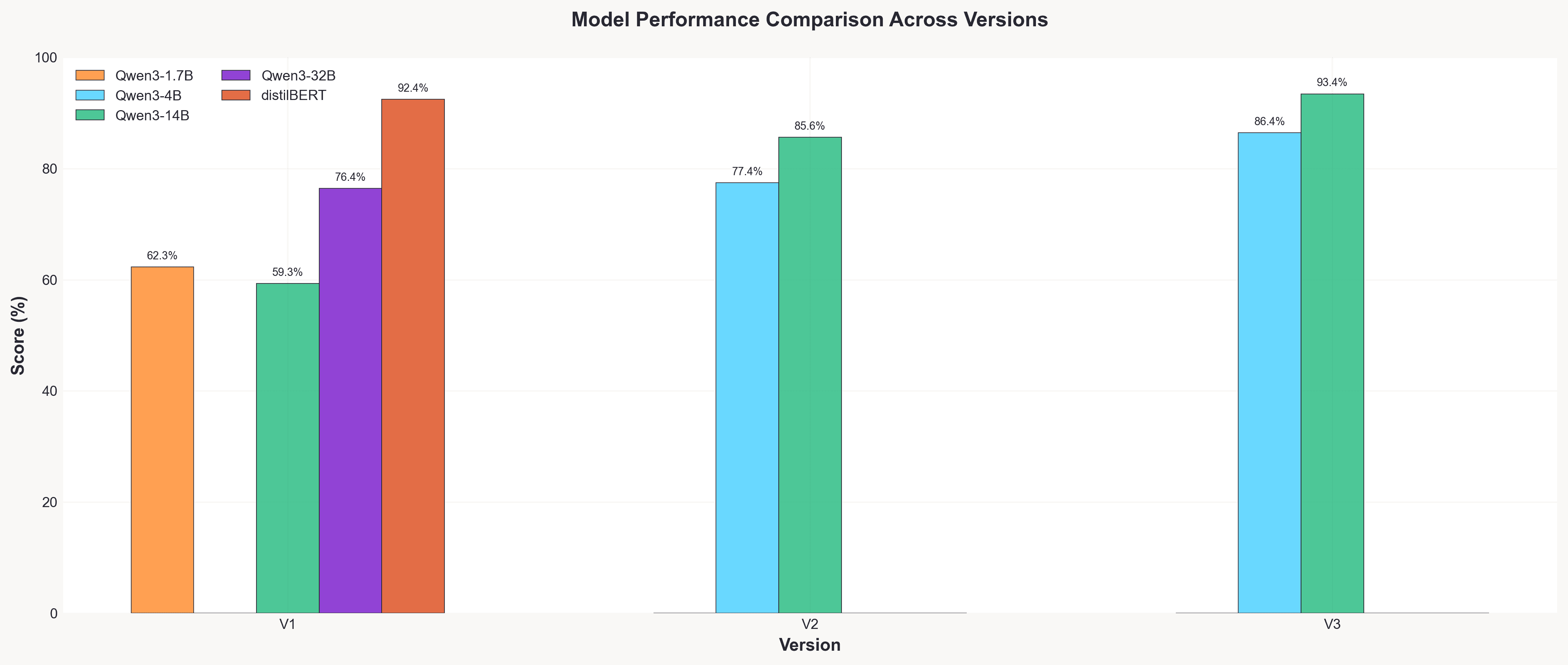
Prompt Version Performance for fine-tuned models
The reasoning prompt rescued struggling classes. On Qwen3-4B, the “Other” category went from 0% F1 (complete failure) to 71% F1 with V3. Science and Arts recall jumped 27-29 percentage points. The reasoning step forces the model to articulate why before committing to a classification, particularly valuable for ambiguous cases.
This was our biggest learning: prompt engineering delivered gains comparable to 5-10x model scaling. Don’t assume the model will learn all categories based on data; spell them out, and make the model show its work. Especially with LoRA, where you are not touching most of the model, these LLM best practices hold.
The Final Push: Scaling Up
With 8,000 balanced examples and the V3 prompt, our fine-tuned models hit their stride:
Model | Accuracy | F1 (macro) | Balanced Acc |
|---|---|---|---|
Qwen3-14B (FT) | 93.42% | 90.75% | 90.28% |
GPT-4.1-nano (FT) | 93.34% | 92.44% | 93.02% |
DistilBERT | 92.43% | 92.63% | 93.32% |
Qwen3-4B (FT) | 86.40% | 81.66% | 82.37% |
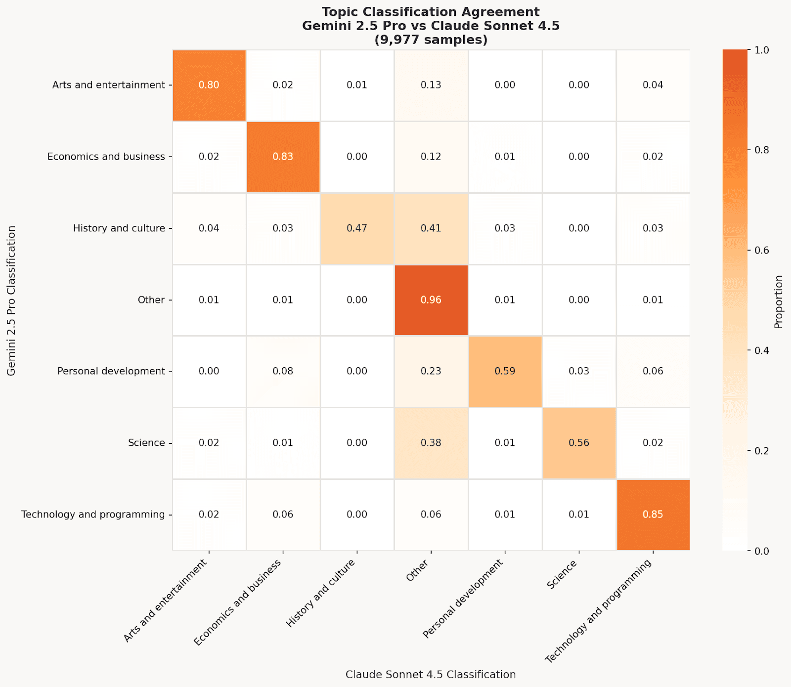
Even our best model had weak spots. The confusion matrix reveals Personal Development (79% F1) struggles because queries about “career planning” blur with Economics. For Personal Development specifically, Gemini and Claude agreed only 43.8% of the time, far below the 77.8% overall agreement rate. The “Other” catch-all also underperforms (83% F1) as models prefer confident specific predictions.
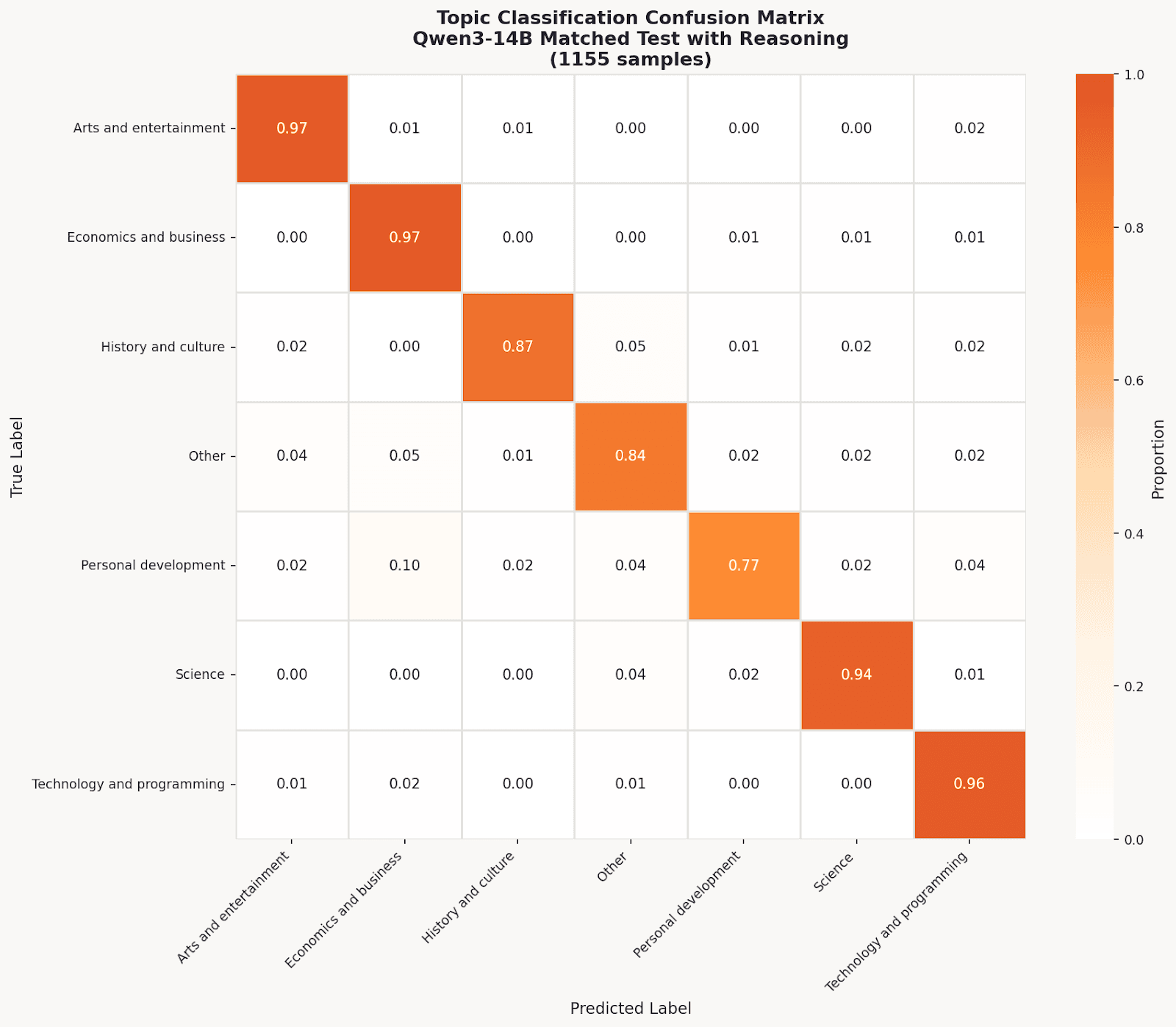
Qwen3-14B Confusion Matrix
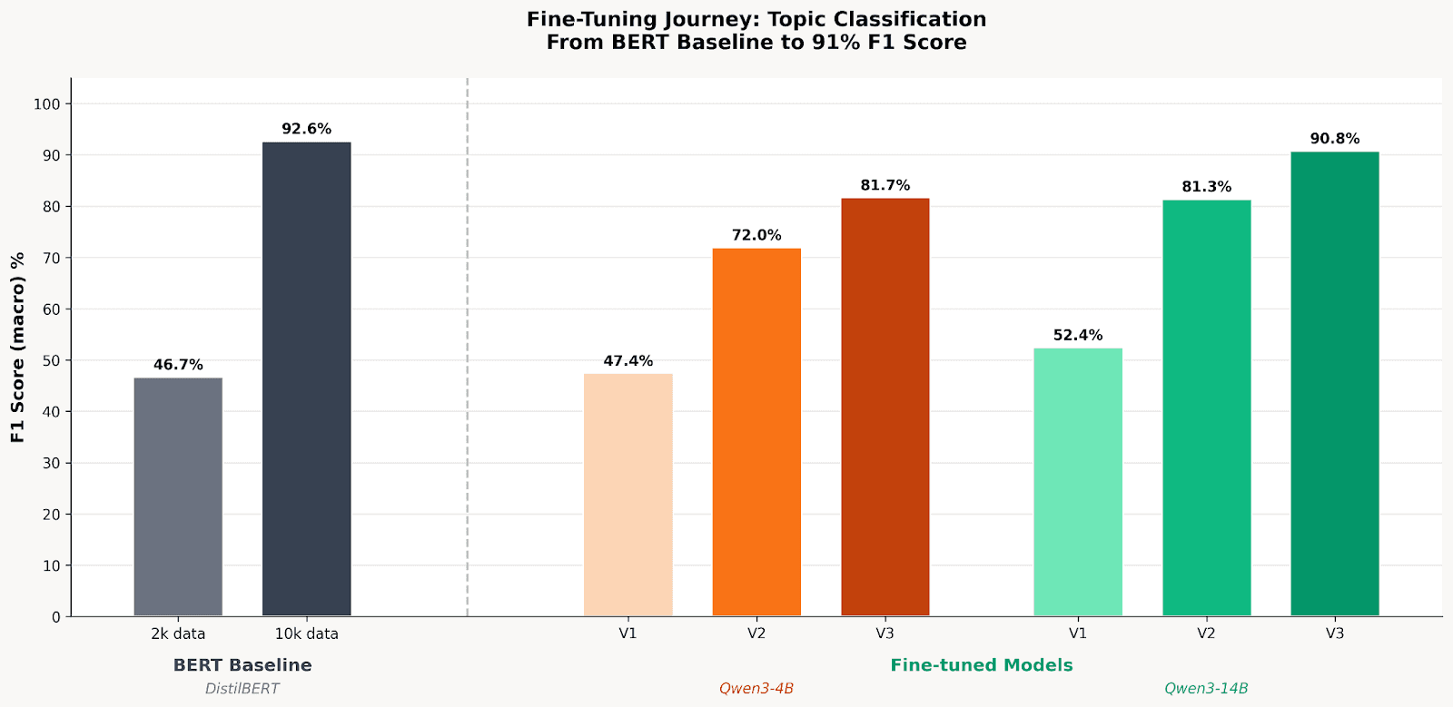
Fine-Tuning Journey: From BERT Baseline to 91% F1
These results didn’t come easily and the data behind them required its own engineering effort.
The Data Challenge
Good agentic datasets are rare. We used the Toucan 1.5M dataset, a collection of synthetic traces generated by running prompts through Kimi K2, GPT-OSS-120B, and Qwen3-32B with various MCP server combinations. With 1.5M traces available and fine-tuning typically requiring 5-10k examples, we had plenty to work with.
We classified only the first user message (not full conversations) because first queries are ~50x shorter (median 62 vs 3,457 tokens), making them compatible with BERT’s 512-token limit while keeping classification consistent across architectures.
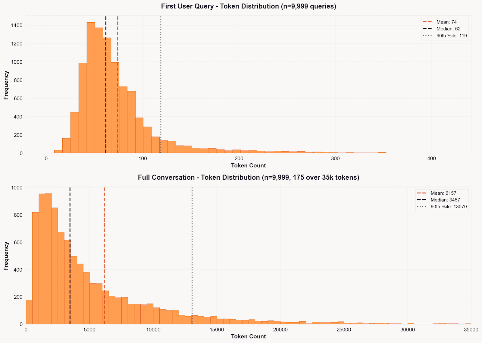
Token Distribution: First Query vs Full Conversation
The Labeling Problem
Human labeling 8k+ samples wasn’t feasible, so we used dual-LLM labeling: Gemini 2.5 Pro and Claude Sonnet 4.5 independently labeled each sample.
Why two models? They’re “differently opinionated.” Sonnet is more conservative (uses “Other” 2.8x more often overall, and 46.8x more often when the models disagree), while Gemini assigns specific categories more confidently. We only kept samples where both models agreed: 77.8% agreement rate (Cohen’s Kappa: 0.72, substantial agreement).
To understand the labeling behaviour of models, it’s interesting to look at where they differ the most in their classifications.
Pattern | Count | Notes |
|---|---|---|
Science → Other (Gemini → Sonnet) | 574 | Sonnet more conservative |
Economics → Other | 259 | |
History → Other | 237 | |
Technology → Economics | 209 | Category boundary confusion |
Gemini vs Claude Agreement
Labeling costs:
Model | Cost | Cost/1k samples |
|---|---|---|
Gemini 2.5 Pro | $4.53 | $0.45 |
Claude Sonnet 4.5 | $21.63 | $2.17 |
Total | $26.16 | $2.62 |
Why the cost difference? Neither model was prompted to reason; both were asked to output only JSON classification. Gemini complied with minimal output (~12 tokens/sample). Claude, lacking native structured output at the time (November 2024), included brief chain-of-thought reasoning before the JSON (~89 tokens/sample average). This reasoning was stripped during post-processing, but the tokens were still billed.
At $2.62/1k samples for labeling vs $0.135-$0.35/1k for fine-tuned inference, the economics strongly favor fine-tuning for high-volume classification—fine-tuned models are 7-19x cheaper per inference than the dual-model labeling cost.
The Imbalance Problem
The Toucan dataset skews heavily toward tool-use interactions, meaning Technology and Programming dominated (40%+ after labeling). Personal Development was just 1.8%.
The dataset’s MCP servers aren’t uniformly distributed: progressing sequentially shifts you between domains (weather tools → finance tools), creating sampling bias. We tried sampling by MCP server category first, but this actually made label imbalance worse.
Final solution: aggressive up/down-sampling to reduce max imbalance from 23:1 to 3.8:1. Not perfect, but workable. We kept the validation set unbalanced to measure real-world performance.
The limitation of upsampling: Starting at 1.8% (Personal Development), even 8x duplication only reaches ~15% representation. Models continue to struggle with minority classes despite our best balancing efforts, as seen in Personal Development’s persistently lower F1 scores across all models.
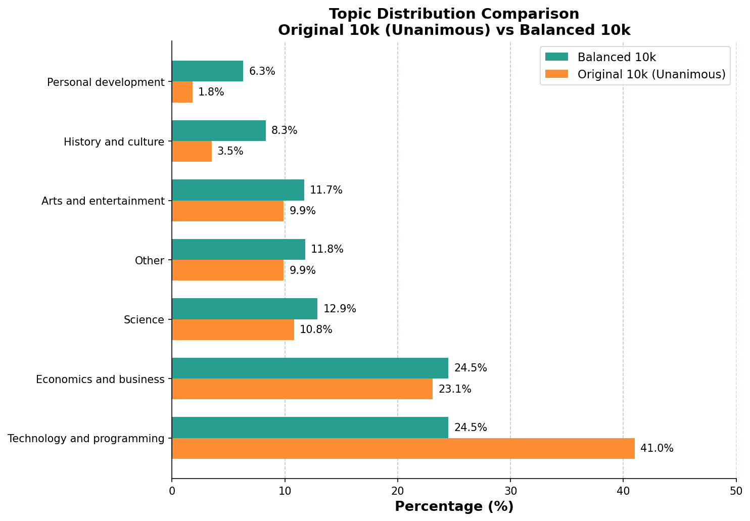
Topic Distribution Before/After
With data in hand, we turned to the practical question: which platform should you actually use for fine-tuning and deployment?
Platform Considerations
Together.ai vs OpenAI
Metric | Together.ai (Qwen3-14B) | OpenAI (GPT-4.1-nano) |
|---|---|---|
Duration | 28 min | 3 hrs |
Training cost | $19.81 | $48.00 |
Inference cost | $0.40/1k (dedicated) | $0.135/1k (serverless) |
Deployment | Dedicated endpoint (manual) | Serverless (instant) |
Control | Full (LoRA rank, weights) | Limited (epochs, batch, LR) |
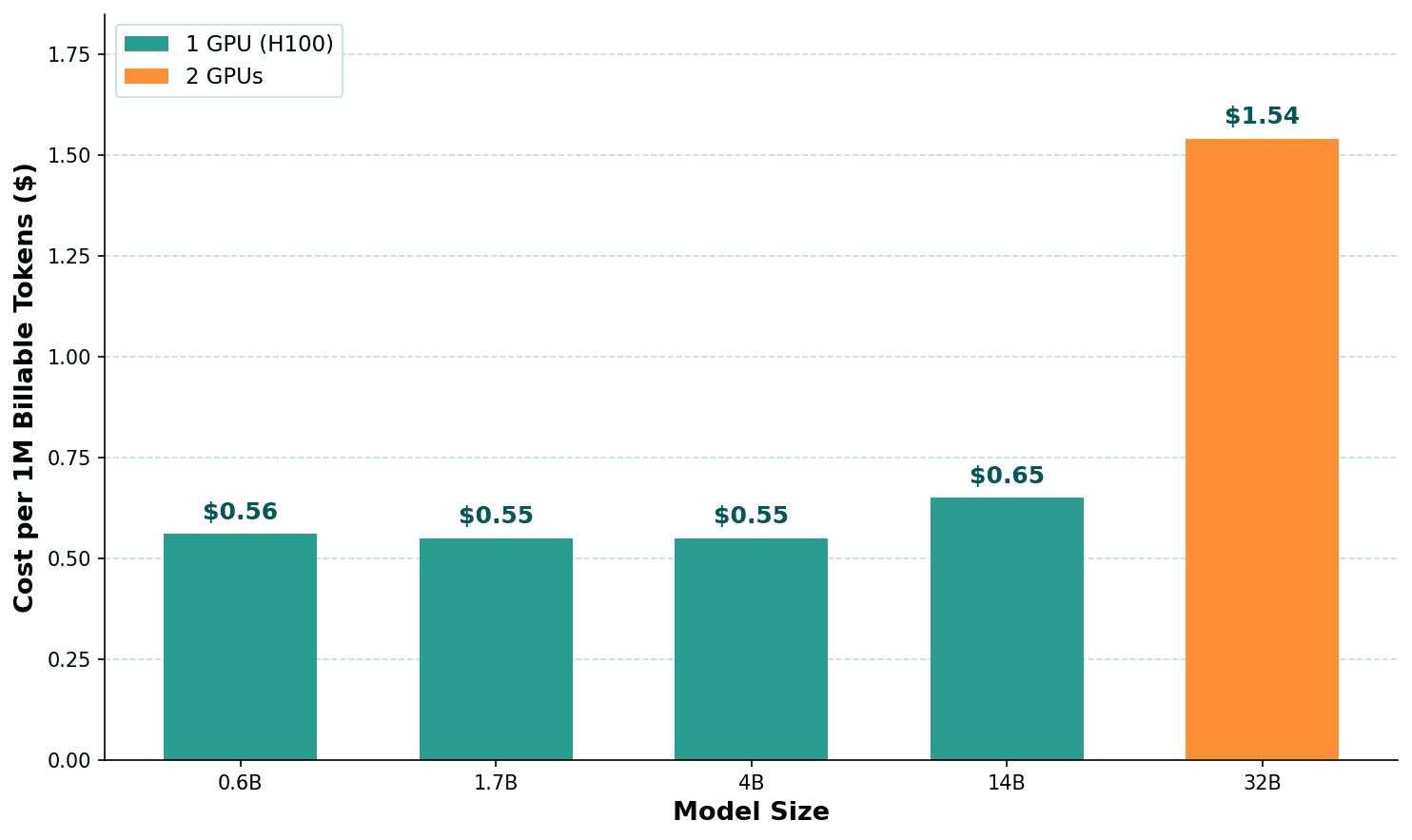
Together.ai charges per billable token (~$0.55/M), not compute time. This means model size barely affects training cost: we paid the same to fine-tune 4B and 14B on identical datasets. The savings are in inference, not training.
When to choose OpenAI: Serverless deployment without GPU management, moderate inference volume (<1M/month), or simplest path to production. GPT-4.1-nano matched accuracy (93.3% vs 93.4%) with better F1 (92.4% vs 90.8%), and inference is 3x cheaper than a dedicated endpoint.
When to choose Together.ai: Full control over training (LoRA rank, adapter weights), faster iteration (6x faster training), or plans to self-host.
Training Cost vs Model Size
Inference Costs: Where Model Size Matters
Unlike training, inference costs scale significantly with model size. Here’s where the 4B sweet spot becomes clear:
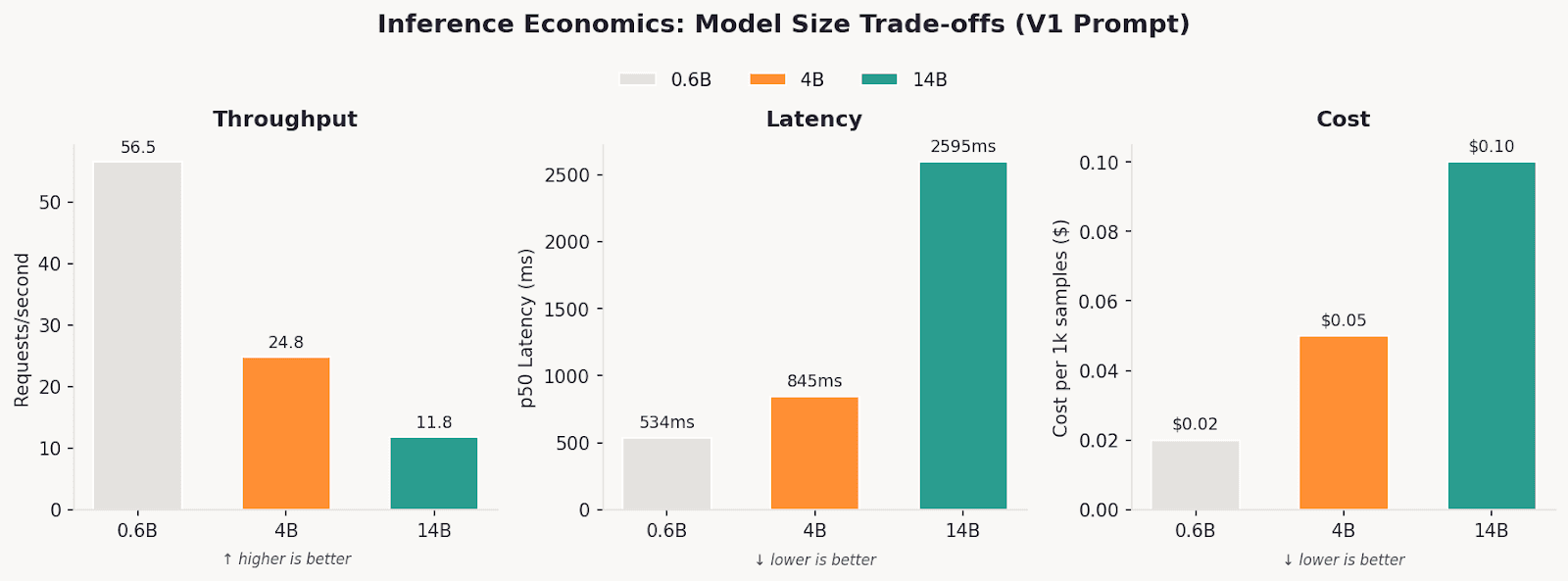
Throughput, latency, and cost scale predictably with model size. 4B offers the best balance: 2.1x faster and 2x cheaper than 14B while achieving 86% accuracy.
Reasoning prompts are expensive: V3 prompts (with reasoning) account for 77% of total inference cost despite having the same number of samples. Why? Output token explosion—reasoning prompts increased output from 10-40 tokens (V1) to 95-358 tokens (V3), a 2-36x increase depending on model. See Appendix D for the full breakdown.
Key insight: Prompt version matters more than model size for latency; output tokens dominate response time, not input tokens. V3’s reasoning field can offset the speed gains of using a smaller model.
Throughput comparison: On V1 prompts, 0.6B achieves 56.5 req/s vs 11.8 req/s for 14B, a 5x difference. But with V3 reasoning prompts, both slow dramatically: 0.6B drops to 9.7 req/s and 14B to 3.1 req/s.
Reliability at Scale
Expect failures with reasoning prompts. When we hit our dedicated endpoints with 50 concurrent async requests using V3 prompts, both 4B and 14B started dropping requests. The 14B showed 96.6% success rate (45 failures out of 1,307) due to long responses triggering timeouts.
Lesson: Implement retry logic with exponential backoff. Reasoning prompts generate unpredictably long outputs. Budget for 2-3 retries per request in production.
Serverless vs Fine-Tuned: The Cost-Accuracy Trade-off
How does fine-tuning compare to just using larger serverless base models?
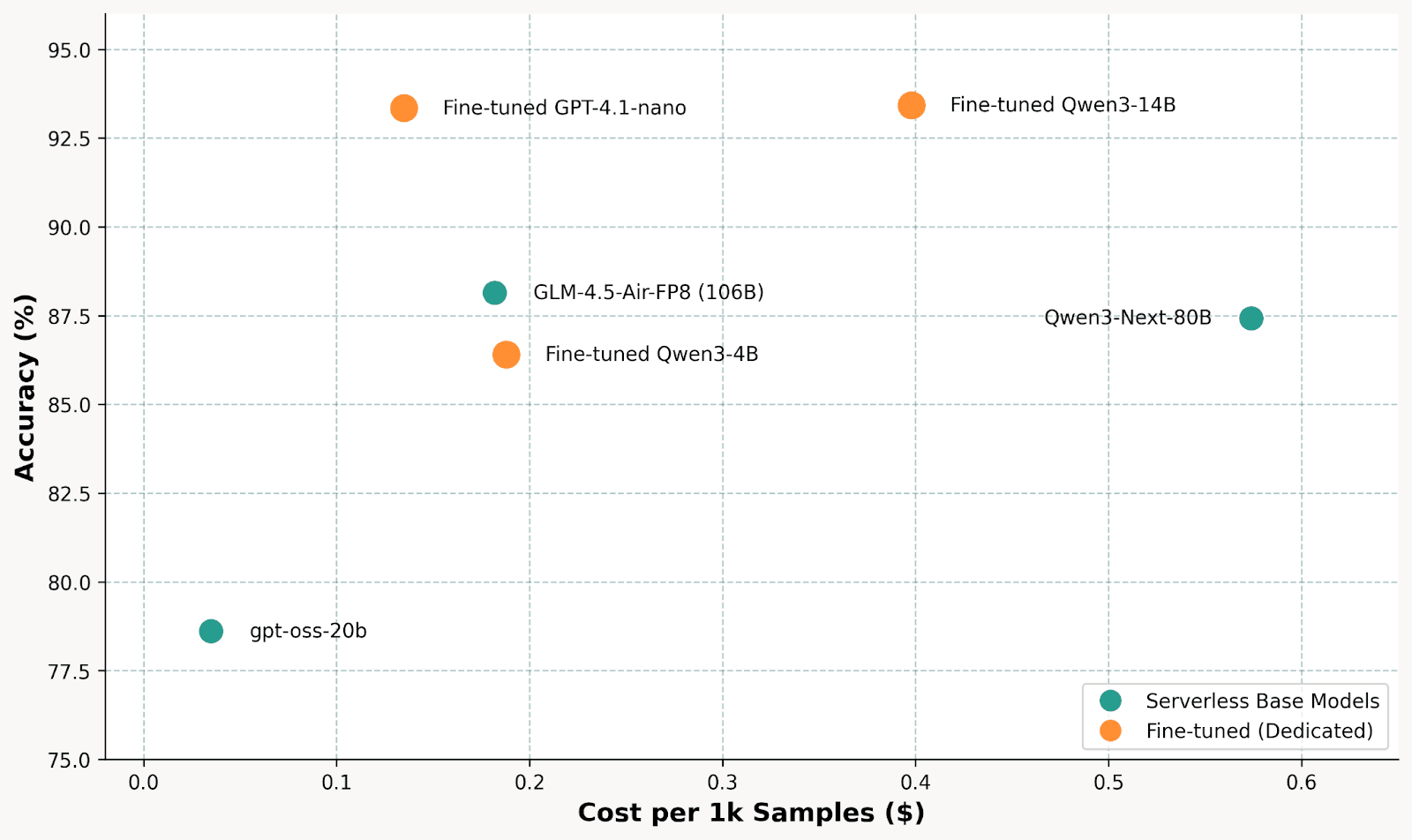
Cost vs Accuracy Trade-off
The fine-tuned 14B dominates the top-right quadrant (high accuracy, moderate cost). It achieves 93.4% accuracy at $0.40/1k samples, beating the 106B GLM model (88%) that costs half as much but sacrifices 5+ points of accuracy. The fine-tuned 4B offers an interesting middle ground at 86.4% accuracy for just $0.19/1k samples. Meanwhile, the 80B Qwen3-Next costs $0.57/1k for only 87.4% accuracy, demonstrating that raw parameter count doesn’t guarantee performance. The real killer here though, is GPT-4.1-nano, delivering equal performance to Qwen3-14B, but doing it much cheaper.
Takeaway: For serverless base models, GLM-4.5-Air-FP8 offers the best cost-accuracy balance. But fine-tuned models win overall: GPT-4.1-nano for serverless simplicity ($0.135/1k, 93.3%), or Qwen3-14B/4B on dedicated endpoints for maximum control.
Note: These costs are for unquantized models on dedicated endpoints. Quantization (e.g., INT8 or INT4) could significantly reduce inference costs while maintaining most of the accuracy. This is a promising direction for further optimization.
Structured Output + Reasoning Models add challenge
Reasoning models (Qwen3-Next, GLM-4.5) are trained to output <reasoning>...</reasoning> tags. But structured output forces JSON. The conflict manifests as:
Models inject XML into JSON: {"reasoning": "<reasoning>...</reasoning>"}
Or have XML before JSON: <reasoning>...</reasoning>{"reasoning": ""}. This happened especially in json_mode, rather than json_schema, where it does not force the model to output the correct structure.
V3’s explicit reasoning field solved this by giving models a sanctioned place to think within the JSON schema, and models adhered surprisingly well. The reasoning traces were the ones from Sonnet 4.5.
The Answer
So to the question: “Could a well-tuned small model match, or beat, models 10x its size?” - Yes, with caveats. Our fine-tuned 14B matched DistilBERT’s accuracy and beat off-the-shelf 80B+ models by 5+ percentage points. The 4B came surprisingly close at half the inference cost.
But this only works for fixed categories. Our actual production need is dynamic classification (user-defined categories that evolve), which this approach can’t handle without retraining. This research validates the fixed-category baseline: when categories stabilize, we know fine-tuning works.
When to Fine-Tune (Checklist)
Fine-tune when:
You have 5k+ labeled examples (ideally 500+ per class)
Categories are stable and won’t change frequently
You need consistent output formatting
Latency is critical (<100ms per request)
You’re processing high volume (cost amortization)
Skip fine-tuning when:
Few-shot prompting already achieves >85% accuracy
Dataset is <2k samples or categories change frequently
You need to handle arbitrary/dynamic categories
DistilBERT vs Fine-Tuned LLMs
DistilBERT deserves special mention. Despite being 60-200x smaller, it matched our best fine-tuned model on balanced metrics—see the Final Push comparison above. DistilBERT actually achieved better macro F1 (92.63% vs 90.75%) and balanced accuracy (93.32% vs 90.28%).
The trade-off: DistilBERT has a 512-token input limit. Our first-message-only approach worked, but if you need to classify longer texts, LLMs are your only option.
Practical Recommendations
Try prompt engineering before scaling up. It delivered our largest accuracy gains
Use 4B for cost-efficiency, 14B for max accuracy. Training cost is the same; pick based on your inference cost trade-off
Start with fewer classes. Our 7-class classification worked; 56-class failed
Data quantity matters. Aim for 500+ samples per class minimum
Consider dual-LLM labeling for cost-effective dataset creation while reducing bias. It should not replace humans, but it’s better than 1 LLM.
Test structured output early. Reasoning models can conflict with JSON schemas
Budget for reasoning tokens. They significantly increase inference costs, but lead to higher performance.
Budget for dual-LLM labeling. It’s cheap and effective
Future Research
Smaller models: Can 1.7B or 0.6B reach 85%+ with more training data?
Hierarchical classification: Predict topic first, then subtopic conditioned on topic
Dynamic categories: Embedding + clustering instead of supervised fine-tuning
Confidence thresholding: Route low-confidence predictions to human review
Evaluate cheaper serverless options: Benchmark Gemini 2.5 Flash ($0.30/$2.50 per 1M tokens) and Claude Haiku 4.5 ($1.00/$5.00 per 1M tokens) to understand their cost-accuracy trade-off compared to the fine-tuned models and serverless base models we tested.
Questions or want to discuss? Reach out to the Orq research team.
Appendix A: Fine-Tuned Model Results
Model | Prompt | Samples Eval | Accuracy | F1 (macro) | Balanced Acc | Precision | Recall |
|---|---|---|---|---|---|---|---|
Qwen3-14B | V3 | 1,155 | 93.42% | 90.75% | 90.28% | 91.32% | 90.28% |
GPT-4.1-nano | V3 | 1,307 | 93.34% | 92.44% | 93.02% | 91.99% | 93.02% |
DistilBERT | - | 1,307 | 92.43% | 92.63% | 93.32% | 92.08% | 93.32% |
Qwen3-4B | V3 | 1,147 | 86.40% | 81.66% | 82.37% | 81.44% | 82.37% |
Qwen3-14B | V2 | 1,154 | 85.62% | 81.35% | 80.73% | 86.38% | 80.73% |
Qwen3-4B | V2 | 1,155 | 77.40% | 71.97% | 71.32% | 75.73% | 71.32% |
Qwen3-1.7B | V1 | - | 62.28% | 49.03% | 49.15% | 65.05% | 49.15% |
Qwen3-14B | V1 | 973 | 59.30% | 52.41% | 51.48% | 65.87% | 51.48% |
Qwen3-4B | V1 | 100 | 58.00% | 47.44% | 54.60% | 47.98% | 54.60% |
DistilBERT | 2k | 996 | 56.22% | 46.67% | 50.77% | 45.95% | 50.77% |
Appendix B: Together.ai Pricing Model
Model Size | Cost/M Billable Tokens | Hardware |
|---|---|---|
0.6B - 14B | ~$0.55/M | 1x H100 80GB |
32B+ | ~$1.65/M | 2x H100 80GB |
Key Finding: Cost per billable token is flat (~$0.55/M) regardless of model size from 0.6B to 14B. Model size does NOT affect cost as long as it fits on the same number of GPUs.
Cost Estimation Formula:
estimated_cost = base_tokens × epochs × $0.55 / 1,000,000
Example: 350K base tokens × 10 epochs = 3.5M billable tokens × $0.55 = $19.25
Appendix C: Topic Distribution (Original vs Balanced)
Topic | Original % | Balanced % | Train | Val |
|---|---|---|---|---|
Technology and programming | 40%+ | ~17% | ~1,100 | 309 |
Economics and business | ~15% | ~17% | ~1,100 | 304 |
Science | ~12% | ~14% | ~900 | 163 |
Arts and entertainment | ~10% | ~12% | ~750 | 132 |
History and culture | ~8% | ~9% | ~550 | 95 |
Other | ~7% | ~9% | ~550 | 100 |
Personal development | 1.8% | ~7% | ~450 | 52 |
Imbalance ratio: 23:1 (original) → 3.8:1 (balanced)
Token Statistics
Metric | First Query | Full Conversation |
|---|---|---|
Median tokens | 62 | 3,457 |
Ratio | 1x | ~50x longer |
We spent weeks fine-tuning 8+ language models on a text classification task, from tiny 0.6B models to 14B behemoths. The question:
Could a well-tuned small model match, or beat, models 10x its size?
The answer surprised us, and the lessons learned apply far beyond our specific use case. While we do our best, this is not an academic paper, but rather a practical, empirical account of what we tried, what failed, and what you can apply to your own fine-tuning projects.
Glossary
This post assumes familiarity with ML fundamentals (training/validation splits, classification metrics) and basic LLM concepts. Here’s a quick glossary:
Term | Definition |
|---|---|
Parameters (4B, 14B) | The number of learnable weights in a model that roughly correlates with capability and cost |
Fine-tuning | Training an existing model on task-specific data to improve performance on that task |
LoRA | Low-Rank Adaptation, which trains only 1-5% of model weights, dramatically reducing memory and compute requirements |
Prompt engineering | Designing input text/instructions to improve model output without changing model weights |
The Business Need
At Orq.ai, we process thousands of conversational traces daily. Understanding what users are discussing (technology questions, business inquiries, creative requests) can give valuable insights to clients. Manual classification doesn’t scale. We needed automated topic classification that’s fast, accurate, and cost-effective.
The Technical Challenge
Text classification sounds simple until you try it. We started with 7 main categories (Technology, Science, Arts, Economics, Personal Development, History, Other) and initially attempted 56 subtopics. The boundaries are fuzzy: is “AI ethics” Technology, Science, or Personal Development? Is “startup funding” Economics or Technology?
Our Goal
Could we fine-tune a 4B or 14B parameter model to beat larger base models? If so, we’d get faster inference, lower costs, and the ability to self-host. The prize: production-quality classification at a fraction of the cost.
The Baseline: What We Were Trying to Beat
We chose the Qwen3 model family for a specific reason: it offers a wide range of sizes (0.6B to 235B) within the same architecture. This let us isolate the effect of model scaling without confounding variables like different tokenizers or training approaches.
Our fine-tuning setup:
Method: LoRA (Low-Rank Adaptation), which trains only 1-5% of model weights
Configuration: Rank 16, alpha 8, learning rate 0.0002
Platform: Together.ai for most runs, OpenAI for comparison
DistilBERT as Floor
Every ML project needs a baseline. DistilBERT (66M parameters) is the classic choice for text classification: small, fast, well-understood. On our 8k balanced dataset, it achieved 92.43% accuracy with 92.63% macro F1.
Why so high? DistilBERT trains all its weights during fine-tuning, not just 1-5% like LoRA. Its encoder architecture is also optimized for understanding tasks like classification. This set a surprisingly high bar: any fine-tuned LLM would need to match a model 60-200x smaller.
Large Base Models as Ceiling
Model | Parameters | Accuracy |
|---|---|---|
GLM-4.5-Air-FP8 | 106B | 88% |
Qwen3-Next-80B | 80B | 87% |
gpt-oss-20b | 20B | 79% |
Even 80-106B models maxed out around 88% without fine-tuning. The ceiling wasn’t as high as we expected, and DistilBERT was already beating them.
With baselines established, we started fine-tuning and quickly learned that the path to 93% accuracy wasn’t straight.
Experiment 1: Topic + Subtopic Classification
We started by trying to do both topic and subtopic classification in one pass.
The prompt:
System: "Classify the topic and subtopic. Provide JSON with fields: topic, subtopic."
User: <query>
Assistant: {"topic"
We thought that fine-tuning would teach the model to map inputs to 7 topics and 56 subtopics, just like any ML classifier learns decision boundaries.
What happened instead was a drop in accuracy across all models. The 56-class problem was too complex; models confused similar subtopics constantly. History vs Culture, Economics vs Business, Science vs Technology boundaries were chaos. We started with 500 datapoints, realized that was much too low, then scaled to 2k data points. However, 56 classes meant ~35 samples each, so still not enough signal. We needed to simplify.
Experiment 2: Simplify to Topic-Only
Dropping subtopics immediately helped. With the same 2k dataset and 7 classes instead of 56 we achieved the following results:
Model | Accuracy Topic + Subtopic | Accuracy Topic |
|---|---|---|
Qwen3-0.6B | 46.9% | 52.1% (+5.2%) |
DistilBERT | 43.3% | 57.4% (+14.1%) |
With topic-only classification working, we scaled up to 8k samples. Model size scaling showed diminishing returns past 4B: moving from 0.6B→1.7B gained +21%, and 1.7B→4B gained +24% (the inflection point), but 4B→14B only added +7%. More strikingly, fine-tuned 14B beat the off-the-shelf 80B base model by 6%.
Why smaller models fail: We tested Qwen3-1.7B and saw a characteristic pattern: very high precision (65%) but low recall (49%). The model becomes ultra-conservative: it achieves 93% recall on Technology (over-predicting the majority class) while minority classes like Personal Development collapse to 14% recall. Below ~4B parameters, models lack the capacity to learn nuanced category boundaries.
What we learned:
Good to restate: start simple, iterate up. Don’t try to solve the hardest version of your problem first.
Our tests were done with a fixed LoRA config, which made 4B the minimum viable size for this task complexity; smaller models fall back to majority-class predictions. With different LoRA configs which touch more weights during fine-tuning, we likely could get similar performance with smaller models.
XML vs JSON: We tested both output formats. XML had similar accuracy but cost ~10% more tokens. JSON won.
Experiment 3: The Prompt Engineering Insight
This is where things got interesting. We iterated on three prompt versions:
V1 (Base):
System: "Classify the topic of the following user query.
Provide your response as JSON with field: topic."
User: <query>
V2 (With Topic List):
System: "Classify the topic. Valid topics:
- Technology and programming
- Science
- Arts and entertainment
- Economics and business
- Personal development
- History and culture
- Other

Provide your response as JSON with field: topic."
User: <
V3 (Topics + Reasoning):
System: [Same as V2, plus:]
"Analyze the query carefully and provide your reasoning before classification.
Provide your response as JSON with fields: reasoning, topic."
User: <query>
The results:
Transition Prompt Versions | Accuracy Gain |
|---|---|
V1 → V2 | +26% (60.4% → 85%) |
V2 → V3 | +8% |
Total | +34% |
Performance gains for Qwen3-14B throughout the prompt versions.
Prompt Version Performance for fine-tuned models
The reasoning prompt rescued struggling classes. On Qwen3-4B, the “Other” category went from 0% F1 (complete failure) to 71% F1 with V3. Science and Arts recall jumped 27-29 percentage points. The reasoning step forces the model to articulate why before committing to a classification, particularly valuable for ambiguous cases.
This was our biggest learning: prompt engineering delivered gains comparable to 5-10x model scaling. Don’t assume the model will learn all categories based on data; spell them out, and make the model show its work. Especially with LoRA, where you are not touching most of the model, these LLM best practices hold.
The Final Push: Scaling Up
With 8,000 balanced examples and the V3 prompt, our fine-tuned models hit their stride:
Model | Accuracy | F1 (macro) | Balanced Acc |
|---|---|---|---|
Qwen3-14B (FT) | 93.42% | 90.75% | 90.28% |
GPT-4.1-nano (FT) | 93.34% | 92.44% | 93.02% |
DistilBERT | 92.43% | 92.63% | 93.32% |
Qwen3-4B (FT) | 86.40% | 81.66% | 82.37% |
Even our best model had weak spots. The confusion matrix reveals Personal Development (79% F1) struggles because queries about “career planning” blur with Economics. For Personal Development specifically, Gemini and Claude agreed only 43.8% of the time, far below the 77.8% overall agreement rate. The “Other” catch-all also underperforms (83% F1) as models prefer confident specific predictions.
Qwen3-14B Confusion Matrix
Fine-Tuning Journey: From BERT Baseline to 91% F1
These results didn’t come easily and the data behind them required its own engineering effort.
The Data Challenge
Good agentic datasets are rare. We used the Toucan 1.5M dataset, a collection of synthetic traces generated by running prompts through Kimi K2, GPT-OSS-120B, and Qwen3-32B with various MCP server combinations. With 1.5M traces available and fine-tuning typically requiring 5-10k examples, we had plenty to work with.
We classified only the first user message (not full conversations) because first queries are ~50x shorter (median 62 vs 3,457 tokens), making them compatible with BERT’s 512-token limit while keeping classification consistent across architectures.
Token Distribution: First Query vs Full Conversation
The Labeling Problem
Human labeling 8k+ samples wasn’t feasible, so we used dual-LLM labeling: Gemini 2.5 Pro and Claude Sonnet 4.5 independently labeled each sample.
Why two models? They’re “differently opinionated.” Sonnet is more conservative (uses “Other” 2.8x more often overall, and 46.8x more often when the models disagree), while Gemini assigns specific categories more confidently. We only kept samples where both models agreed: 77.8% agreement rate (Cohen’s Kappa: 0.72, substantial agreement).
To understand the labeling behaviour of models, it’s interesting to look at where they differ the most in their classifications.
Pattern | Count | Notes |
|---|---|---|
Science → Other (Gemini → Sonnet) | 574 | Sonnet more conservative |
Economics → Other | 259 | |
History → Other | 237 | |
Technology → Economics | 209 | Category boundary confusion |
Gemini vs Claude Agreement
Labeling costs:
Model | Cost | Cost/1k samples |
|---|---|---|
Gemini 2.5 Pro | $4.53 | $0.45 |
Claude Sonnet 4.5 | $21.63 | $2.17 |
Total | $26.16 | $2.62 |
Why the cost difference? Neither model was prompted to reason; both were asked to output only JSON classification. Gemini complied with minimal output (~12 tokens/sample). Claude, lacking native structured output at the time (November 2024), included brief chain-of-thought reasoning before the JSON (~89 tokens/sample average). This reasoning was stripped during post-processing, but the tokens were still billed.
At $2.62/1k samples for labeling vs $0.135-$0.35/1k for fine-tuned inference, the economics strongly favor fine-tuning for high-volume classification—fine-tuned models are 7-19x cheaper per inference than the dual-model labeling cost.
The Imbalance Problem
The Toucan dataset skews heavily toward tool-use interactions, meaning Technology and Programming dominated (40%+ after labeling). Personal Development was just 1.8%.
The dataset’s MCP servers aren’t uniformly distributed: progressing sequentially shifts you between domains (weather tools → finance tools), creating sampling bias. We tried sampling by MCP server category first, but this actually made label imbalance worse.
Final solution: aggressive up/down-sampling to reduce max imbalance from 23:1 to 3.8:1. Not perfect, but workable. We kept the validation set unbalanced to measure real-world performance.
The limitation of upsampling: Starting at 1.8% (Personal Development), even 8x duplication only reaches ~15% representation. Models continue to struggle with minority classes despite our best balancing efforts, as seen in Personal Development’s persistently lower F1 scores across all models.
Topic Distribution Before/After
With data in hand, we turned to the practical question: which platform should you actually use for fine-tuning and deployment?
Platform Considerations
Together.ai vs OpenAI
Metric | Together.ai (Qwen3-14B) | OpenAI (GPT-4.1-nano) |
|---|---|---|
Duration | 28 min | 3 hrs |
Training cost | $19.81 | $48.00 |
Inference cost | $0.40/1k (dedicated) | $0.135/1k (serverless) |
Deployment | Dedicated endpoint (manual) | Serverless (instant) |
Control | Full (LoRA rank, weights) | Limited (epochs, batch, LR) |
Together.ai charges per billable token (~$0.55/M), not compute time. This means model size barely affects training cost: we paid the same to fine-tune 4B and 14B on identical datasets. The savings are in inference, not training.
When to choose OpenAI: Serverless deployment without GPU management, moderate inference volume (<1M/month), or simplest path to production. GPT-4.1-nano matched accuracy (93.3% vs 93.4%) with better F1 (92.4% vs 90.8%), and inference is 3x cheaper than a dedicated endpoint.
When to choose Together.ai: Full control over training (LoRA rank, adapter weights), faster iteration (6x faster training), or plans to self-host.
Training Cost vs Model Size
Inference Costs: Where Model Size Matters
Unlike training, inference costs scale significantly with model size. Here’s where the 4B sweet spot becomes clear:
Throughput, latency, and cost scale predictably with model size. 4B offers the best balance: 2.1x faster and 2x cheaper than 14B while achieving 86% accuracy.
Reasoning prompts are expensive: V3 prompts (with reasoning) account for 77% of total inference cost despite having the same number of samples. Why? Output token explosion—reasoning prompts increased output from 10-40 tokens (V1) to 95-358 tokens (V3), a 2-36x increase depending on model. See Appendix D for the full breakdown.
Key insight: Prompt version matters more than model size for latency; output tokens dominate response time, not input tokens. V3’s reasoning field can offset the speed gains of using a smaller model.
Throughput comparison: On V1 prompts, 0.6B achieves 56.5 req/s vs 11.8 req/s for 14B, a 5x difference. But with V3 reasoning prompts, both slow dramatically: 0.6B drops to 9.7 req/s and 14B to 3.1 req/s.
Reliability at Scale
Expect failures with reasoning prompts. When we hit our dedicated endpoints with 50 concurrent async requests using V3 prompts, both 4B and 14B started dropping requests. The 14B showed 96.6% success rate (45 failures out of 1,307) due to long responses triggering timeouts.
Lesson: Implement retry logic with exponential backoff. Reasoning prompts generate unpredictably long outputs. Budget for 2-3 retries per request in production.
Serverless vs Fine-Tuned: The Cost-Accuracy Trade-off
How does fine-tuning compare to just using larger serverless base models?
Cost vs Accuracy Trade-off
The fine-tuned 14B dominates the top-right quadrant (high accuracy, moderate cost). It achieves 93.4% accuracy at $0.40/1k samples, beating the 106B GLM model (88%) that costs half as much but sacrifices 5+ points of accuracy. The fine-tuned 4B offers an interesting middle ground at 86.4% accuracy for just $0.19/1k samples. Meanwhile, the 80B Qwen3-Next costs $0.57/1k for only 87.4% accuracy, demonstrating that raw parameter count doesn’t guarantee performance. The real killer here though, is GPT-4.1-nano, delivering equal performance to Qwen3-14B, but doing it much cheaper.
Takeaway: For serverless base models, GLM-4.5-Air-FP8 offers the best cost-accuracy balance. But fine-tuned models win overall: GPT-4.1-nano for serverless simplicity ($0.135/1k, 93.3%), or Qwen3-14B/4B on dedicated endpoints for maximum control.
Note: These costs are for unquantized models on dedicated endpoints. Quantization (e.g., INT8 or INT4) could significantly reduce inference costs while maintaining most of the accuracy. This is a promising direction for further optimization.
Structured Output + Reasoning Models add challenge
Reasoning models (Qwen3-Next, GLM-4.5) are trained to output <reasoning>...</reasoning> tags. But structured output forces JSON. The conflict manifests as:
Models inject XML into JSON: {"reasoning": "<reasoning>...</reasoning>"}
Or have XML before JSON: <reasoning>...</reasoning>{"reasoning": ""}. This happened especially in json_mode, rather than json_schema, where it does not force the model to output the correct structure.
V3’s explicit reasoning field solved this by giving models a sanctioned place to think within the JSON schema, and models adhered surprisingly well. The reasoning traces were the ones from Sonnet 4.5.
The Answer
So to the question: “Could a well-tuned small model match, or beat, models 10x its size?” - Yes, with caveats. Our fine-tuned 14B matched DistilBERT’s accuracy and beat off-the-shelf 80B+ models by 5+ percentage points. The 4B came surprisingly close at half the inference cost.
But this only works for fixed categories. Our actual production need is dynamic classification (user-defined categories that evolve), which this approach can’t handle without retraining. This research validates the fixed-category baseline: when categories stabilize, we know fine-tuning works.
When to Fine-Tune (Checklist)
Fine-tune when:
You have 5k+ labeled examples (ideally 500+ per class)
Categories are stable and won’t change frequently
You need consistent output formatting
Latency is critical (<100ms per request)
You’re processing high volume (cost amortization)
Skip fine-tuning when:
Few-shot prompting already achieves >85% accuracy
Dataset is <2k samples or categories change frequently
You need to handle arbitrary/dynamic categories
DistilBERT vs Fine-Tuned LLMs
DistilBERT deserves special mention. Despite being 60-200x smaller, it matched our best fine-tuned model on balanced metrics—see the Final Push comparison above. DistilBERT actually achieved better macro F1 (92.63% vs 90.75%) and balanced accuracy (93.32% vs 90.28%).
The trade-off: DistilBERT has a 512-token input limit. Our first-message-only approach worked, but if you need to classify longer texts, LLMs are your only option.
Practical Recommendations
Try prompt engineering before scaling up. It delivered our largest accuracy gains
Use 4B for cost-efficiency, 14B for max accuracy. Training cost is the same; pick based on your inference cost trade-off
Start with fewer classes. Our 7-class classification worked; 56-class failed
Data quantity matters. Aim for 500+ samples per class minimum
Consider dual-LLM labeling for cost-effective dataset creation while reducing bias. It should not replace humans, but it’s better than 1 LLM.
Test structured output early. Reasoning models can conflict with JSON schemas
Budget for reasoning tokens. They significantly increase inference costs, but lead to higher performance.
Budget for dual-LLM labeling. It’s cheap and effective
Future Research
Smaller models: Can 1.7B or 0.6B reach 85%+ with more training data?
Hierarchical classification: Predict topic first, then subtopic conditioned on topic
Dynamic categories: Embedding + clustering instead of supervised fine-tuning
Confidence thresholding: Route low-confidence predictions to human review
Evaluate cheaper serverless options: Benchmark Gemini 2.5 Flash ($0.30/$2.50 per 1M tokens) and Claude Haiku 4.5 ($1.00/$5.00 per 1M tokens) to understand their cost-accuracy trade-off compared to the fine-tuned models and serverless base models we tested.
Questions or want to discuss? Reach out to the Orq research team.
Appendix A: Fine-Tuned Model Results
Model | Prompt | Samples Eval | Accuracy | F1 (macro) | Balanced Acc | Precision | Recall |
|---|---|---|---|---|---|---|---|
Qwen3-14B | V3 | 1,155 | 93.42% | 90.75% | 90.28% | 91.32% | 90.28% |
GPT-4.1-nano | V3 | 1,307 | 93.34% | 92.44% | 93.02% | 91.99% | 93.02% |
DistilBERT | - | 1,307 | 92.43% | 92.63% | 93.32% | 92.08% | 93.32% |
Qwen3-4B | V3 | 1,147 | 86.40% | 81.66% | 82.37% | 81.44% | 82.37% |
Qwen3-14B | V2 | 1,154 | 85.62% | 81.35% | 80.73% | 86.38% | 80.73% |
Qwen3-4B | V2 | 1,155 | 77.40% | 71.97% | 71.32% | 75.73% | 71.32% |
Qwen3-1.7B | V1 | - | 62.28% | 49.03% | 49.15% | 65.05% | 49.15% |
Qwen3-14B | V1 | 973 | 59.30% | 52.41% | 51.48% | 65.87% | 51.48% |
Qwen3-4B | V1 | 100 | 58.00% | 47.44% | 54.60% | 47.98% | 54.60% |
DistilBERT | 2k | 996 | 56.22% | 46.67% | 50.77% | 45.95% | 50.77% |
Appendix B: Together.ai Pricing Model
Model Size | Cost/M Billable Tokens | Hardware |
|---|---|---|
0.6B - 14B | ~$0.55/M | 1x H100 80GB |
32B+ | ~$1.65/M | 2x H100 80GB |
Key Finding: Cost per billable token is flat (~$0.55/M) regardless of model size from 0.6B to 14B. Model size does NOT affect cost as long as it fits on the same number of GPUs.
Cost Estimation Formula:
estimated_cost = base_tokens × epochs × $0.55 / 1,000,000
Example: 350K base tokens × 10 epochs = 3.5M billable tokens × $0.55 = $19.25
Appendix C: Topic Distribution (Original vs Balanced)
Topic | Original % | Balanced % | Train | Val |
|---|---|---|---|---|
Technology and programming | 40%+ | ~17% | ~1,100 | 309 |
Economics and business | ~15% | ~17% | ~1,100 | 304 |
Science | ~12% | ~14% | ~900 | 163 |
Arts and entertainment | ~10% | ~12% | ~750 | 132 |
History and culture | ~8% | ~9% | ~550 | 95 |
Other | ~7% | ~9% | ~550 | 100 |
Personal development | 1.8% | ~7% | ~450 | 52 |
Imbalance ratio: 23:1 (original) → 3.8:1 (balanced)
Token Statistics
Metric | First Query | Full Conversation |
|---|---|---|
Median tokens | 62 | 3,457 |
Ratio | 1x | ~50x longer |

